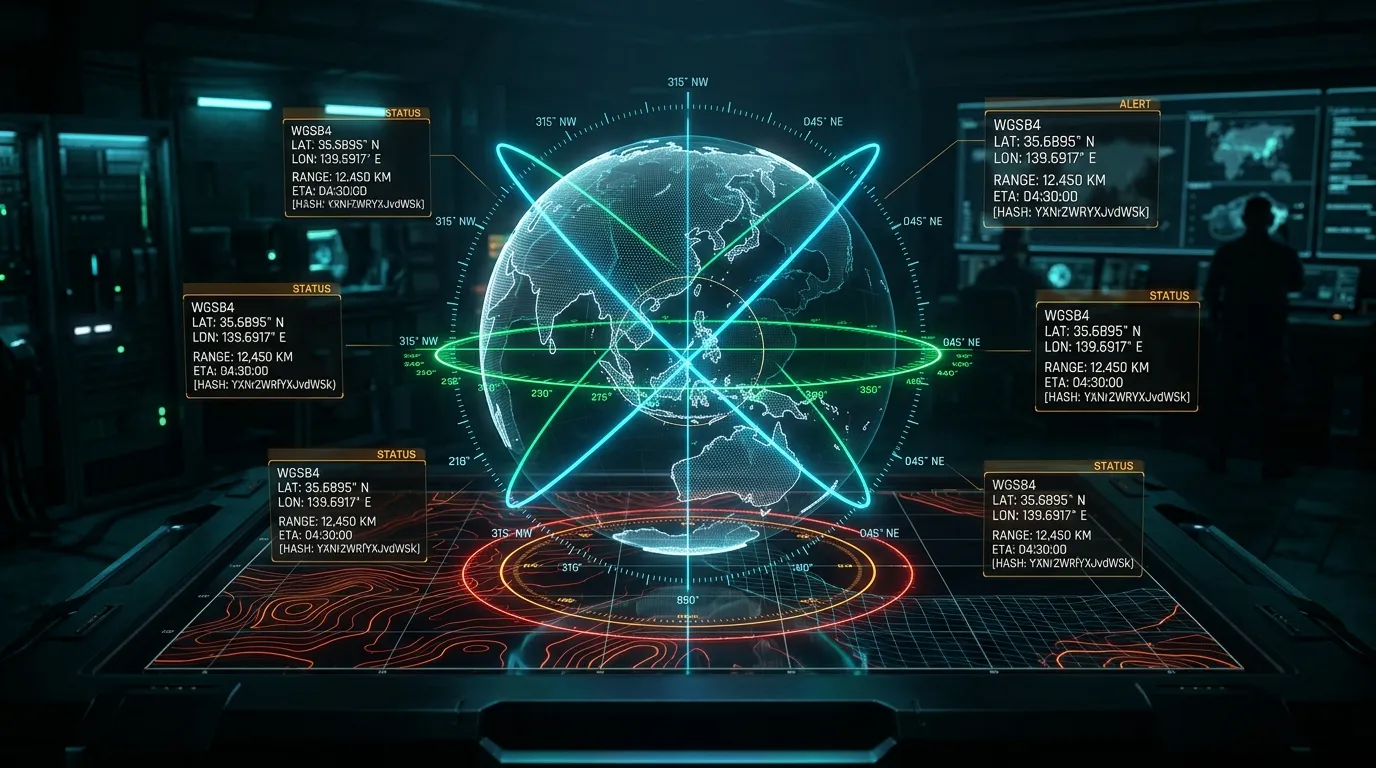
Coordy: Zero-Backend Geodesic Vector Plotting, WMM2025 Declination & URL-Hash State Compression

Whether you are aligning long-range directional LoRa or point-to-point microwave antennas, triangulating RF signal sources during a wireless foxhunt, navigating by physical lensatic compass in GPS-denied environments, or verifying azimuth sightlines in an open-source intelligence (OSINT) investigation, calculating accurate forward, arrival, and reverse bearings across multiple geographic coordinates is a daily operational requirement.

Yet nearly every web-based mapping and azimuth utility forces a painful trade-off: either require cloud user accounts, log every coordinate pair you query to third-party analytics servers, draw misleading flat-Mercator lines that ignore Earth’s curvature, or persist shared multi-vector maps inside a centralized backend database.

We built Coordy (GitHub: Tekromancy/coordy) to solve this with radical simplicity: a 100% client-side, zero-backend geodesic vector plotter and tactical compass calculator built with Next.js, OpenStreetMap, and Leaflet. Every great-circle orthodrome, constant-heading Rhumb loxodrome, World Magnetic Model (WMM2025) magnetic declination angle, forward destination projection, and Slerp geodesic curve is computed locally in your browser—and entire multi-vector map topologies (including camera center, zoom level, active basemap, and custom labels) can be shared via compact base64url URI fragments (#v=...) or exported to GeoJSON, GPX, KML, and CSV without a single coordinate ever touching a server log.

Explore the live application at coordy.tekromancy.com or experiment with the interactive Geodesic & WMM2025 simulator embedded at the bottom of this dispatch.

1. Tri-Mode Geodesic Engine: Orthodrome vs. Loxodrome vs. Planar 2D

A pervasive trap in naive geospatial scripts is treating latitude ($\phi$) and longitude ($\lambda$) as a flat Euclidean grid ($dx = \Delta\lambda,; dy = \Delta\phi$), or assuming that a straight line drawn on a Web Mercator (EPSG:3857) map represents the shortest physical path on Earth. Outside the equator, meridian convergence ($\cos\phi$) warps flat-plane angles severely.

Even more subtly, a Great-Circle path (orthodrome) and a constant-compass-heading Rhumb line (loxodrome) diverge dramatically over medium-to-long baselines:

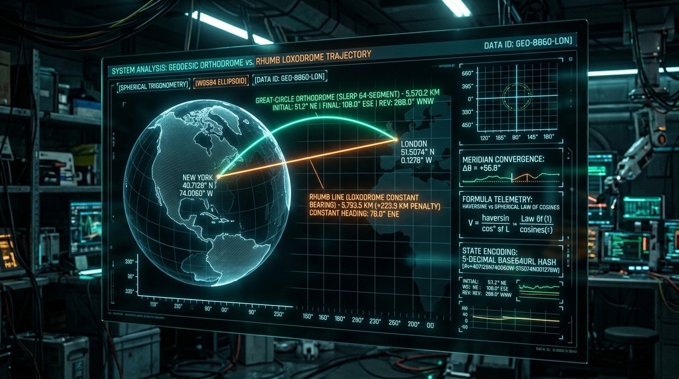
1. Great-Circle Orthodrome (geographic): The shortest physical distance between two points on a sphere ($R = 6,371.0088\text{ km}$, per the IUGG mean Earth radius). Because meridians converge toward the poles, your forward compass heading continuously shifts along the trajectory. Flying from New York ($40.7128^\circ\text{ N}, 74.0060^\circ\text{ W}$) to London ($51.5074^\circ\text{ N}, 0.1278^\circ\text{ W}$) begins at an initial bearing of $51.2^\circ\text{ (NE)}$, arcs northward toward Greenland, and arrives in London at a final bearing of $108.0^\circ\text{ (ESE)}$—a meridian convergence shift of $+56.8^\circ$! Consequently, the true reverse bearing from London back to New York is $288.0^\circ\text{ (WNW)}$, whereas the naive flat-plane formula $(\theta_1 + 180^\circ) \bmod 360^\circ = 231.2^\circ$ is wrong by nearly $57^\circ$.
2. Rhumb Line / Loxodrome (rhumb): A path of constant compass heading that crosses every meridian at the exact same angle. On a Web Mercator projection, a Rhumb line appears as a straight Euclidean segment. Steering a constant $78.0^\circ\text{ (ENE)}$ from New York to London requires zero heading adjustments, but adds a $+223.3\text{ km}$ distance penalty ($5,793.5\text{ km}$ vs. $5,570.2\text{ km}$).
3. Planar 2D Cartesian (planar): Pure Euclidean vector geometry ($\theta = \text{atan2}(\Delta x, \Delta y) \bmod 360^\circ$) for flat CTF grids, local CAD site plans, and compatibility with our compass.py challenge scripts.

+-------------------------------------------------------------------------------+
|         TRI-MODE AZIMUTH ENGINE: ORTHODROME vs. LOXODROME vs. PLANAR          |
+-------------------------------------------------------------------------------+
|                                                                               |
|                      North Pole (Meridian Convergence)                        |
|                                     /\                                        |
|          Initial Bearing (θ₁=51.2°)/  \  Final Arrival Bearing (θ_end=108.0°) |
|                 \                 /    \                 /                    |
|                  v      Slerp Great-Circle Arc          v                     |
|                  _.•*˜˜*•._      /      \      _.•*˜˜*•._                     |
|       [ Point A ] =========*====/========\====*=========> [ Point B ]         |
|      (NYC: φ₁,λ₁) \            /          \              (LON: φ₂,λ₂)         |
|                    \__________/____________\____________/                     |
|                       Rhumb Line (Constant ψ = 78.0° ENE)                     |
|                                                                               |
|  * Great-Circle (geographic): Shortest surface arc; true reverse θ_BA != θ₁+π |
|  * Rhumb Line   (rhumb):      Constant Mercator heading via isometric Δψ      |
|  * Planar 2D    (planar):     Flat Cartesian atan2(Δx, Δy) & √(Δx² + Δy²)     |
+-------------------------------------------------------------------------------+

Inside src/lib/bearing.ts: True Reverse Bearing & Isometric Rhumb Math

In src/lib/bearing.ts, Coordy computes all three modes natively. For Geographic Mode, it evaluates both the forward spherical law of cosines from $A \to B$ and the inverted spherical azimuth from $B \to A$ to derive the exact True Reverse Bearing (backBearing) and Final Arrival Bearing (finalBearing):

export type CalculationMode = 'geographic' | 'rhumb' | 'planar';

export interface BearingResult {
  mode: CalculationMode;
  bearing: number;              // 0 to 360° (initial heading at Point A)
  finalBearing?: number;        // 0 to 360° (arrival heading at Point B)
  backBearing: number;          // 0 to 360° (true reverse heading Point B -> Point A)
  cardinal: string;             // e.g. "NNE", "SSW"
  cardinalName: string;         // e.g. "North-Northeast"
  distanceKm?: number;
  distanceMiles?: number;
  distanceNauticalMiles?: number;
  distanceMeters?: number;
  distanceFeet?: number;
  dx?: number;
  dy?: number;
  magneticBearing?: number;
  magneticBackBearing?: number;
  magneticDeclination?: number; // at Point A origin
}

const EARTH_RADIUS_KM = 6371.0088; // IUGG mean Earth radius

export function calculateGeographicBearing(p1: Coordinate, p2: Coordinate): BearingResult {
  const phi1 = toRadians(p1.lat);
  const phi2 = toRadians(p2.lat);
  const deltaLambda = toRadians(p2.lon - p1.lon);

  // Initial bearing from p1 to p2
  const y = Math.sin(deltaLambda) * Math.cos(phi2);
  const x =
    Math.cos(phi1) * Math.sin(phi2) -
    Math.sin(phi1) * Math.cos(phi2) * Math.cos(deltaLambda);
  const bearing = (toDegrees(Math.atan2(y, x)) + 360) % 360;

  // True reverse initial bearing from p2 to p1 (meridian convergence accounted for)
  const yRev = Math.sin(-deltaLambda) * Math.cos(phi1);
  const xRev =
    Math.cos(phi2) * Math.sin(phi1) -
    Math.sin(phi2) * Math.cos(phi1) * Math.cos(-deltaLambda);
  const backBearing = (toDegrees(Math.atan2(yRev, xRev)) + 360) % 360;

  // Final bearing arriving at p2
  const finalBearing = (backBearing + 180) % 360;

  // Haversine great-circle distance
  const deltaPhi = toRadians(p2.lat - p1.lat);
  const a =
    Math.sin(deltaPhi / 2) * Math.sin(deltaPhi / 2) +
    Math.cos(phi1) * Math.cos(phi2) * Math.sin(deltaLambda / 2) * Math.sin(deltaLambda / 2);
  const c = 2 * Math.atan2(Math.sqrt(a), Math.sqrt(1 - a));

  const distanceKm = EARTH_RADIUS_KM * c;
  const distanceMiles = distanceKm * 0.62137119;
  const distanceNauticalMiles = distanceKm / 1.852;
  const distanceMeters = distanceKm * 1000;
  const distanceFeet = distanceMeters * 3.28084;

  const cardinal = getCardinalDirection(bearing);

  // Compute local magnetic declination at origin p1 via WMM2025
  let magneticBearing: number | undefined;
  let magneticBackBearing: number | undefined;
  let magneticDeclination: number | undefined;

  try {
    magneticDeclination = calculateMagneticDeclination(p1.lat, p1.lon);
    magneticBearing = trueToMagnetic(bearing, magneticDeclination);
    const declinationP2 = calculateMagneticDeclination(p2.lat, p2.lon);
    magneticBackBearing = trueToMagnetic(backBearing, declinationP2);
  } catch {
    // Fallback if magnetic calculation fails
  }

  return {
    mode: 'geographic',
    bearing,
    finalBearing,
    backBearing,
    cardinal: cardinal.code,
    cardinalName: cardinal.name,
    distanceKm,
    distanceMiles,
    distanceNauticalMiles,
    distanceMeters,
    distanceFeet,
    magneticBearing,
    magneticBackBearing,
    magneticDeclination,
  };
}

For Rhumb Line (Loxodrome) Mode, Coordy projects latitudes onto the Mercator isometric latitude parameter $\Delta\psi = \ln\left(\frac{\tan(\pi/4 + \phi_2/2)}{\tan(\pi/4 + \phi_1/2)}\right)$, handling both East-West parallel runs ($\Delta\psi \to 0 \implies q = \cos\phi_1$) and International Date Line anti-meridian wrap-around ($|\Delta\lambda| > \pi$):

export function calculateRhumbBearing(p1: Coordinate, p2: Coordinate): BearingResult {
  const phi1 = toRadians(p1.lat);
  const phi2 = toRadians(p2.lat);
  let deltaLambda = toRadians(p2.lon - p1.lon);

  // Shortest path across the 180° antimeridian
  if (Math.abs(deltaLambda) > Math.PI) {
    deltaLambda = deltaLambda > 0 ? -(2 * Math.PI - deltaLambda) : 2 * Math.PI + deltaLambda;
  }

  const deltaPhi = phi2 - phi1;
  const deltaPsi = Math.log(
    Math.tan(Math.PI / 4 + phi2 / 2) / Math.tan(Math.PI / 4 + phi1 / 2)
  );

  const q = Math.abs(deltaPsi) > 1e-12 ? deltaPhi / deltaPsi : Math.cos(phi1);
  const bearing = (toDegrees(Math.atan2(deltaLambda, deltaPsi)) + 360) % 360;
  const backBearing = (bearing + 180) % 360;

  const angularDist = Math.sqrt(deltaPhi * deltaPhi + q * q * deltaLambda * deltaLambda);
  const distanceKm = angularDist * EARTH_RADIUS_KM;

  const cardinal = getCardinalDirection(bearing);

  return {
    mode: 'rhumb',
    bearing,
    finalBearing: bearing, // Rhumb heading is constant along entire route
    backBearing,
    cardinal: cardinal.code,
    cardinalName: cardinal.name,
    distanceKm,
    distanceMiles: distanceKm * 0.62137119,
    distanceNauticalMiles: distanceKm / 1.852,
    distanceMeters: distanceKm * 1000,
    distanceFeet: distanceKm * 1000 * 3.28084,
  };
}

2. Spherical Linear Interpolation (Slerp) & Forward Destination Projection

If you pass two coordinates [p1, p2] directly to a standard Leaflet L.polyline(), Leaflet draws a straight Euclidean segment on the Web Mercator canvas—which visually represents a flat Rhumb line rather than the true Great-Circle path. Over long transoceanic or high-latitude baselines, a straight Mercator line departs from the true physical ground track by hundreds of kilometers.

Geodesic Slerp Curves (interpolateGreatCircle)

To render true curved orthodromes on the map without third-party plugins, Coordy implements Spherical Linear Interpolation (Slerp) in src/lib/bearing.ts. Given angular distance $\Omega$ between unit vectors on the sphere, intermediate fractions $f = i / N$ across $N$ segments are projected in 3D Cartesian space and converted back to spherical $(\phi_i, \lambda_i)$:

$$\text{Slerp}(\vec{v}_1, \vec{v}_2, f) = \frac{\sin((1 - f)\Omega)}{\sin\Omega}\vec{v}_1 + \frac{\sin(f\Omega)}{\sin\Omega}\vec{v}_2$$

export function interpolateGreatCircle(
  p1: [number, number],
  p2: [number, number],
  numSegments = 32
): [number, number][] {
  const lat1 = toRadians(p1[0]);
  const lon1 = toRadians(p1[1]);
  const lat2 = toRadians(p2[0]);
  const lon2 = toRadians(p2[1]);

  // Convert to 3D Cartesian unit vectors
  const v1 = [
    Math.cos(lat1) * Math.cos(lon1),
    Math.cos(lat1) * Math.sin(lon1),
    Math.sin(lat1),
  ];
  const v2 = [
    Math.cos(lat2) * Math.cos(lon2),
    Math.cos(lat2) * Math.sin(lon2),
    Math.sin(lat2),
  ];

  const dot = v1[0] * v2[0] + v1[1] * v2[1] + v1[2] * v2[2];
  const clampedDot = Math.max(-1, Math.min(1, dot));
  const omega = Math.acos(clampedDot);

  if (Math.abs(omega) < 1e-6) {
    return [p1, p2];
  }

  const sinOmega = Math.sin(omega);
  const points: [number, number][] = [];

  for (let i = 0; i <= numSegments; i++) {
    const f = i / numSegments;
    const s1 = Math.sin((1 - f) * omega) / sinOmega;
    const s2 = Math.sin(f * omega) / sinOmega;

    const x = s1 * v1[0] + s2 * v2[0];
    const y = s1 * v1[1] + s2 * v2[1];
    const z = s1 * v1[2] + s2 * v2[2];

    const lat = toDegrees(Math.atan2(z, Math.sqrt(x * x + y * y)));
    const lon = toDegrees(Math.atan2(y, x));

    points.push([lat, lon]);
  }

  return points;
}

In src/components/MapComponent.tsx, Coordy renders this interpolated Slerp polyline on the map, placing the rotating directional arrow and bearing badge directly at the true spherical midpoint ($f = 0.5$).

Forward Geodesic Projection (calculateDestinationPoint)

What if you have an origin coordinate $P_1$, a known azimuth heading $\theta$ (e.g., from a directional Yagi antenna or witness sightline), and an estimated distance $d$? Coordy’s Forward Destination Projection solves the Direct Geodetic Problem across all three calculation modes:

$$\phi_2 = \arcsin\left(\sin\phi_1\cos\delta + \cos\phi_1\sin\delta\cos\theta\right)$$

$$\lambda_2 = \lambda_1 + \text{atan2}\left(\sin\theta\sin\delta\cos\phi_1,; \cos\delta - \sin\phi_1\sin\phi_2\right)$$

export function calculateDestinationPoint(
  start: Coordinate,
  bearingDeg: number,
  distanceKm: number,
  mode: CalculationMode = 'geographic'
): Coordinate {
  if (mode === 'planar') {
    const rad = toRadians(bearingDeg);
    const dx = distanceKm * Math.sin(rad);
    const dy = distanceKm * Math.cos(rad);
    return {
      lat: start.lat + dy,
      lon: start.lon + dx,
    };
  }

  const phi1 = toRadians(start.lat);
  const lambda1 = toRadians(start.lon);
  const theta = toRadians(bearingDeg);
  const delta = distanceKm / EARTH_RADIUS_KM;

  if (mode === 'geographic') {
    const phi2 = Math.asin(
      Math.sin(phi1) * Math.cos(delta) + Math.cos(phi1) * Math.sin(delta) * Math.cos(theta)
    );
    const lambda2 =
      lambda1 +
      Math.atan2(
        Math.sin(theta) * Math.sin(delta) * Math.cos(phi1),
        Math.cos(delta) - Math.sin(phi1) * Math.sin(phi2)
      );

    const latDeg = toDegrees(phi2);
    const lonDeg = ((toDegrees(lambda2) + 540) % 360) - 180;
    return { lat: latDeg, lon: lonDeg };
  } else {
    // Rhumb destination
    const phi2 = phi1 + delta * Math.cos(theta);
    const deltaPsi = Math.log(
      Math.tan(Math.PI / 4 + phi2 / 2) / Math.tan(Math.PI / 4 + phi1 / 2)
    );
    const q = Math.abs(deltaPsi) > 1e-12 ? (phi2 - phi1) / deltaPsi : Math.cos(phi1);
    const deltaLambda = (delta * Math.sin(theta)) / q;
    const lambda2 = lambda1 + deltaLambda;

    const latDeg = toDegrees(phi2);
    const lonDeg = ((toDegrees(lambda2) + 540) % 360) - 180;
    return { lat: latDeg, lon: lonDeg };
  }
}

Inside the Destination Projection tab of src/components/BearingModal.tsx, operators can enter origin $P_1$, heading $\theta$, and distance in km, mi, nm, m, or ft, calculate the destination coordinate, and click Plot Vector on Map to immediately inject the sightline into the active canvas.

3. Offline World Magnetic Model (WMM2025) Declination Engine

Geodesic formulas produce bearings referenced to True Geographic North (the Earth’s rotational spin axis). However, physical lensatic and baseplate compasses align with the local geomagnetic field (Magnetic North). Across North America and Europe, magnetic declination ($\delta$) routinely diverges from True North by $5^\circ$ to $25^\circ$.

Rather than calling external NOAA APIs (which would leak coordinates and fail offline), Coordy embeds a standalone World Magnetic Model (WMM2025) Spherical Harmonic Engine in src/lib/magnetic.ts:

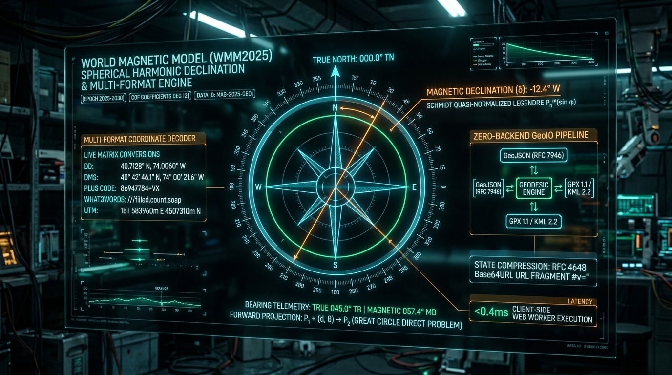
Spherical Harmonics & Schmidt Quasi-Normalized Legendre Polynomials

Coordy models the Earth’s main geomagnetic potential $V(r, \theta, \lambda)$ up to harmonic degree $n = 5$ using the official NOAA/NCEI WMM2025 Gauss coefficients $(g_n^m, h_n^m)$ and secular variation rates $(\dot{g}_n^m, \dot{h}_n^m)$ for epoch $2025.0\text{–}2030.0$:

$$V(r, \theta, \lambda) = a \sum_{n=1}^{5} \left(\frac{a}{r}\right)^{n+1} \sum_{m=0}^{n} \left(g_n^m(t)\cos(m\lambda) + h_n^m(t)\sin(m\lambda)\right) P_n^m(\cos\theta)$$

The surface magnetic field $\vec{B} = -\nabla V$ yields North ($X$) and East ($Y$) components from the gradient:

$$X = \frac{1}{r} \frac{\partial V}{\partial\theta}, \quad Y = -\frac{1}{r\sin\theta} \frac{\partial V}{\partial\lambda}$$

$$\text{Declination } \delta = \text{atan2}(Y, X)$$

Here is the exact implementation in src/lib/magnetic.ts:

interface WMMCoeff {
  n: number;
  m: number;
  g: number;  // nT
  h: number;  // nT
  dg: number; // nT / year
  dh: number; // nT / year
}

const WMM_EPOCH = 2025.0;
const WMM_COEFFS: WMMCoeff[] = [
  // n=1
  { n: 1, m: 0, g: -29404.5, h: 0.0, dg: 6.7, dh: 0.0 },
  { n: 1, m: 1, g: -1450.7, h: 4652.9, dg: 7.7, dh: -25.1 },
  // n=2
  { n: 2, m: 0, g: -2500.0, h: 0.0, dg: -11.5, dh: 0.0 },
  { n: 2, m: 1, g: 2982.0, h: -2991.6, dg: -1.6, dh: -30.2 },
  { n: 2, m: 2, g: 1676.8, h: -734.8, dg: -6.9, dh: -23.9 },
  // n=3..5 degrees
];

function schmidtLegendre(nMax: number, cosTheta: number, sinTheta: number): number[][] {
  const P: number[][] = Array.from({ length: nMax + 1 }, () => Array(nMax + 1).fill(0));
  P[0][0] = 1;

  for (let m = 1; m <= nMax; m++) {
    const factor = m === 1 ? Math.sqrt(2) : Math.sqrt((2 * m - 1) / (2 * m));
    P[m][m] = sinTheta * factor * P[m - 1][m - 1];
  }

  P[1][0] = cosTheta;
  for (let n = 2; n <= nMax; n++) {
    P[n][0] = ((2 * n - 1) / n) * cosTheta * P[n - 1][0] - ((n - 1) / n) * P[n - 2][0];
  }

  for (let m = 1; m <= nMax; m++) {
    for (let n = m + 1; n <= nMax; n++) {
      const K = Math.sqrt(((n - 1) * (n - 1) - m * m) / ((2 * n - 1) * (2 * n - 3)));
      const factor = (2 * n - 1) / Math.sqrt(n * n - m * m);
      P[n][m] = factor * cosTheta * P[n - 1][m] - (factor * K) * P[n - 2][m];
    }
  }

  return P;
}

export function calculateMagneticDeclination(
  lat: number,
  lon: number,
  date: Date = new Date()
): number {
  const currentYear = date.getFullYear() + date.getMonth() / 12 + date.getDate() / 365.25;
  const dt = currentYear - WMM_EPOCH;

  const theta = ((90 - lat) * Math.PI) / 180;
  const lambda = (lon * Math.PI) / 180;
  const eps = 1e-6;

  const dV_dtheta = (calculatePotential(theta + eps, lambda, dt) - calculatePotential(theta - eps, lambda, dt)) / (2 * eps);
  const dV_dlambda = (calculatePotential(theta, lambda + eps, dt) - calculatePotential(theta, lambda - eps, dt)) / (2 * eps);

  const sinTheta = Math.sin(theta);
  const X = dV_dtheta;
  const Y = Math.abs(sinTheta) > 1e-5 ? -dV_dlambda / sinTheta : 0;

  const declinationRad = Math.atan2(Y, X);
  return (declinationRad * 180) / Math.PI;
}

export function trueToMagnetic(trueBearing: number, declinationDeg: number): number {
  return ((trueBearing - declinationDeg) % 360 + 360) % 360;
}

In the Compass Modal (src/components/BearingModal.tsx), Coordy displays both the True Bearing and the Magnetic Bearing ($\theta_{\text{mag}} = (\theta_{\text{true}} - \delta + 360^\circ) \bmod 360^\circ$), complete with the local declination badge (e.g., +4.31° E in Austin or -11.5° W in New York).

4. Universal Coordinate Parsing & Zero-Dependency Plus Codes

Coordinates in field operations arrive in arbitrary notations: Decimal Degrees, aviation DMS (30° 16' 1.9" N, 97° 44' 35.2" W), Degrees Decimal Minutes (30° 16.032' N), Google Open Location Codes / Plus Codes (86247784+Vp), or what3words addresses (///filled.count.soap).

Coordy’s unified parser (src/lib/coordinates.ts) detects and validates all formats automatically.

Zero-Dependency Plus Code Decoder (decodePlusCode)

To decode Google Plus Codes without bundling the official library, Coordy implements a clean base-20 grid decoder:

const OLC_ALPHABET = '23456789CFGHJMPQRVWX';

export function decodePlusCode(code: string): { lat: number; lon: number } | null {
  const cleanCode = code.trim().toUpperCase().replace(/0+$/, '');
  if (!cleanCode.includes('+')) return null;

  const parts = cleanCode.split('+');
  if (parts.length !== 2) return null;
  const fullSeq = (parts[0] + parts[1]).replace(/0/g, '');

  let south = -90;
  let west = -180;
  let latResolution = 20;
  let lonResolution = 20;

  const pairCount = Math.min(Math.floor(fullSeq.length / 2), 5);
  for (let i = 0; i < pairCount; i++) {
    const latVal = OLC_ALPHABET.indexOf(fullSeq[i * 2]);
    const lonVal = OLC_ALPHABET.indexOf(fullSeq[i * 2 + 1]);
    if (latVal === -1 || lonVal === -1) return null;

    south += latVal * latResolution;
    west += lonVal * lonResolution;
    latResolution /= 20;
    lonResolution /= 20;
  }

  // Handle grid refinement if length > 10 characters (4x5 subgrid per char)
  if (fullSeq.length > 10) {
    const extraChars = fullSeq.slice(10);
    for (let i = 0; i < extraChars.length; i++) {
      const idx = OLC_ALPHABET.indexOf(extraChars[i]);
      south += Math.floor(idx / 4) * (latResolution / 5);
      west += (idx % 4) * (lonResolution / 4);
      latResolution /= 5;
      lonResolution /= 4;
    }
  }

  return {
    lat: Math.max(-90, Math.min(90, south + latResolution / 2)),
    lon: Math.max(-180, Math.min(180, west + lonResolution / 2)),
  };
}

Combined with our floating Nominatim Place Search component (src/components/PlaceSearch.tsx), operators can type landmark names, street addresses, Plus Codes, or coordinates, preview geocoded results with 350ms debouncing, and instantly fly to any location.

5. Extended URL-Hash Codec & Multi-Format GeoIO

Coordy serializes complete map states into client-side URL hash fragments (#v=...). Because RFC 3986 fragment identifiers are never transmitted in HTTP GET requests, server logs never receive a single coordinate.

The Extended URL Hash Payload (src/lib/codec.ts)

In coordy, encodeMapStateToHash() serializes not only 5-decimal quantized vector coordinates, but also camera zoom (z), map center (c), calculation mode (m), basemap ID (b), and per-vector labels (l):

export type CompactVector = [number, number, number, number];

export interface SharedMapPayload {
  v: CompactVector[];
  z?: number;
  c?: [number, number];       // [lat, lng]
  m?: CalculationMode;        // 'geographic' | 'rhumb' | 'planar'
  b?: string;                 // basemap id ('dark' | 'osm' | 'topo' | 'satellite')
  l?: string[];               // custom vector labels
}

export function encodeMapStateToHash(
  vectors: MapVector[],
  viewState?: MapViewState,
  mode?: CalculationMode,
  basemap?: string
): string {
  const compact: CompactVector[] = vectors.map((v) => [
    Number(v.from[0].toFixed(5)),
    Number(v.from[1].toFixed(5)),
    Number(v.to[0].toFixed(5)),
    Number(v.to[1].toFixed(5)),
  ]);

  const payload: SharedMapPayload = { v: compact };

  if (viewState) {
    payload.z = Math.round(viewState.zoom * 10) / 10;
    payload.c = [
      Number(viewState.center[0].toFixed(5)),
      Number(viewState.center[1].toFixed(5)),
    ];
  }
  if (mode && mode !== 'geographic') payload.m = mode;
  if (basemap && basemap !== 'osm') payload.b = basemap;
  if (vectors.some((v) => Boolean(v.label))) {
    payload.l = vectors.map((v) => v.label || '');
  }

  const jsonStr = JSON.stringify(payload);
  return btoa(jsonStr).replace(/\+/g, '-').replace(/\//g, '_').replace(/=+$/, '');
}

Full GIS Interoperability (src/lib/geoio.ts)

For integration with ATAK/CivTAK, QGIS, ArcGIS, Google Earth, and handheld GPS units, Coordy provides bidirectional import/export:

• GeoJSON (RFC 7946): Generates a FeatureCollection with Slerp-interpolated LineString coordinates and navigation properties (bearing, cardinal, distanceKm), and imports external GeoJSON files.
• GPX 1.1: Generates GPS route tracks with <rtept> waypoints for Garmin and OsmAnd receivers.
• KML 2.2: Generates Google Earth placemarks with <tessellate>1</tessellate> enabled so great-circle curves hug terrain contours.
• CSV: Exports tabular spreadsheets with coordinates, initial bearings, reverse bearings, and distance metrics in metric, imperial, and nautical miles.

6. Tactical Map Workflows: Basemaps, Chaining & Rubber-Banding

In src/components/MapComponent.tsx and src/app/page.tsx, Coordy provides tactical spatial controls:

1. 4 Live Basemaps: Instant switching between CartoDB Dark Matter (night ops), OpenStreetMap Standard, OpenTopoMap (elevation contour lines for line-of-sight RF profiling), and Esri World Imagery (satellite photography).
2. 60 FPS Geodesic Rubber-Banding: Click origin A to preview a live dashed geodesic arc with real-time bearing and distance badges following the cursor. Click or drag endpoints at any time to dynamically re-aim vectors.
3. Shortest-Arc Compass Needle Physics: The visual compass rose normalizes boundary crossing via (((target - current) % 360) + 540) % 360 - 180, ensuring smooth spring animations (cubic-bezier(0.34, 1.56, 0.64, 1)) across the $360^\circ / 0^\circ$ North threshold.
4. Vector Route Chaining & Direction Inversion: In the Vector Drawer, 1-click Chain (+) starts a new vector leg from the end of an existing vector, while Invert (⇄) swaps start and target endpoints, instantly recalculating all bearings and updating cumulative traverse distance.

Launch the live tool at coordy.tekromancy.com or inspect the open-source repository at github.com/Tekromancy/coordy.